Interactive Data App with Streamlit¶

Open example in Github

We’ll use the TLC NY Taxi dataset TLC NY taxi dataset and build a pipeline that combines data from the Yellow Taxi Records with the Taxi Zone Lookup Table. The pipeline will generate a table named top_pickup_location, which displays the boroughs and zones in New York City with the highest number of taxi pickups. Finally, we’ll use Streamlit to visualize this table in an interactive app.

Set up¶

To begin, install bauplan and `set up your project

Pipeline¶

The final shape of the pipeline is the the following:

flowchart LR id0[(taxi_fhvhv)]-->id2[models.normalized_taxi_trips] id2[models.normalized_taxi_trips] --> id4[models.top_pickup_locations] id3[(taxi_zones)] --> id4[models.top_pickup_locations]

This pipeline has two main components:

trips_and_zones: this function performs two scans on S3 using Python and joins the results with PyArrow. The scans retrieve data from the taxi_fhvhv and taxi_zones tables, filtering records based on pickup timestamps. The join operation aligns taxi trips with their corresponding pickup locations by matching the PULocationID field with LocationID.
top_pickup_locations: this function uses Pandas to aggregate and sort the data from trips_and_zones. It groups taxi trips by PULocationID, Borough, and Zone and orders the results by the total number of trips, producing a table of the most popular pickup locations in New York City.

While it is not mandatory to collect models in a single models.py file, we recommend it as a best practice for keeping the pipeline’s logic centralized and organized. The top_pickup_locations function uses the materialization_strategy='REPLACE' flag to persist the results as an Iceberg table. This materialization makes the data queryable and ready for visualization in Streamlit.

import bauplan

@bauplan.model()
@bauplan.python('3.11')
def trips_and_zones(
        trips=bauplan.Model(
            'taxi_fhvhv',
            # this function does an S3 scan directly in Python, so we can specify the columns and the filter pushdown
            # by pushing the filters down to S3 we make the system considerably more performant
            columns=[
                'pickup_datetime',
                'dropoff_datetime',
                'PULocationID',
                'DOLocationID',
                'trip_miles',
                'trip_time',
                'base_passenger_fare',
                'tips',
            ],
            filter="pickup_datetime >= '2023-01-01T00:00:00-05:00' AND pickup_datetime < '2023-02-02T00:00:00-05:00'"
        ),
        zones=bauplan.Model(
            'taxi_zones',
        ),
):
    """
    this function does an S3 scan over two tables - taxi_fhvhv and zones - filtering by pickup_datetime
    it then joins them over PULocationID and LocationID using Pyarrow https://arrow.apache.org/docs/python/index.html
    the output is a table with the taxi trip the taxi trips in the relevant period and the corresponding pickup Zones
    """

    import math

    # the following code is PyArrow
    # because Bauplan speaks Arrow natively you don't need to import PyArrow explicitly
    # join 'trips' with 'zones' on 'PULocationID' and 'LocationID'
    pickup_location_table = (trips.join(zones, 'PULocationID', 'LocationID').combine_chunks())
    # print the size of the resulting table
    size_in_gb = round(pickup_location_table.nbytes / math.pow(1024, 3), 3)
    print(f"\nThis table is {size_in_gb} GB and has {pickup_location_table.num_rows} rows\n")

    return pickup_location_table


# this function explicitly requires that its output is materialized in the data catalog as an Iceberg table
@bauplan.model(materialization_strategy='REPLACE')
@bauplan.python('3.11', pip={'pandas': '2.2.0'})
def top_pickup_locations(data=bauplan.Model('trips_and_zones')):
    """
    this function takes the parent table with the taxi trips and the corresponding pickup zones
    and groups the taxi trips by PULocationID, Borough and Zone sorting them in descending order
    the output is the table of the top pickup locations by number of trips
    """

    import pandas as pd

    # convert the input Arrow table into a Pandas dataframe
    df = data.to_pandas()

    # group the taxi trips by PULocationID, Borough and Zone and sort in descending order
    # the result will be a Pandas dataframe with all the pickup locations sorted by number of trips
    top_pickup_table = (
        df
        .groupby(['PULocationID', 'Borough', 'Zone'])
        .agg(number_of_trips=('pickup_datetime', 'count'))
        .reset_index()
        .sort_values(by='number_of_trips', ascending=False)
    )
    # we can return a Pandas dataframe
    return top_pickup_table

Run the Pipeline¶

First, create a new branch and switch to it.

bauplan branch create <YOUR_BRANCH>
bauplan branch checkout <YOUR_BRANCH>

Create a bauplan branch and run the pipeline in it so you will have a table in it named top_pickup_locations,

With the new branch checked out, run the pipeline to materialize the table top_pickup_locations.

bauplan run

After the pipeline completes, inspect the newly created top_pickup_locations table in your branch to ensure everything ran successfully.

bauplan table get top_pickup_locations

Streamlit app¶

To visualize the data we will use Streamlit, a powerful Python framework to build web apps in pure Python. The example below contains a Streamlit app to visualize the table top_pickup_location created with the bauplan pipeline above. This simple script shows how to use bauplan’s Python SDK to embed querying and other functionalities in a data app.

import streamlit as st
import sys
from argparse import ArgumentParser
import plotly.express as px
import bauplan
import pandas as pd


@st.cache_data()
def query_as_dataframe(
        _client: bauplan.Client,
        sql: str,
        branch: str
) -> pd.DataFrame:
    """
    Runs a query with bauplan and put the table in a Pandas dataframe
    """
    try:
        df = _client.query(query=sql, ref=branch).to_pandas()
        return df
    except bauplan.exceptions.BauplanError as e:
        print(f"Error: {e}")
        return None


def plot_interactive_chart(df: pd.DataFrame) -> None:
    """
    Creates an interactive bar chart using Plotly Express
    """
    # Define the figure to display in the app
    fig = px.bar(
        df,
        y='Zone',
        x='number_of_trips',
        orientation='h',
        title='Number of Trips per Zone',
        labels={'number_of_trips': 'Number of Trips', 'Zone': 'Zone'},
        height=800
    )

    # Customize the layout
    fig.update_layout(
        showlegend=False,
        xaxis_title="Number of Trips",
        yaxis_title="Zone",
        hoverlabel=dict(bgcolor="white"),
        margin=dict(l=20, r=20, t=40, b=20)
    )

    # Display the plot in Streamlit
    st.plotly_chart(fig, use_container_width=True)


def main():
    # Set up command line argument parsing
    parser = ArgumentParser()
    parser.add_argument('--branch', type=str, required=True, help='Branch name to query data from')
    args = parser.parse_args()

    # set up the table name as a global
    table_name = 'top_pickup_locations'

    st.title('A simple data app to visualize taxi rides and locations in NY')

    # instantiate a bauplan client
    client = bauplan.Client()

    # Using the branch from command line argument
    branch = args.branch

    # Query the table top_pickup_locations using bauplan
    df = query_as_dataframe(
        _client=client,
        sql=f"SELECT * FROM {table_name}",
        branch=branch
    )

    if df is not None and not df.empty:
        # Add a toggle for viewing raw data
        if st.checkbox('Show raw data'):
            st.dataframe(df.head(50), width=1200)

        # Display the interactive plot
        plot_interactive_chart(df=df.head(50))
    else:
        st.error('Error retrieving data. Please check your branch name and try again.')


if __name__ == "__main__":
    main()

Run the Streamlit app¶

Create a virtual environment, install the necessary requirements and then run the Streamlit app. Remember that you will need to pass the branch in which you materialized the target table as an argument in the terminal.

python3 -m venv venv
source venv/bin/activate
pip install bauplan streamlit==1.28.1 pandas==2.2.0 matplotlib==3.8.1 seaborn==0.13.0 plotly==5.24.1
streamlit run viz_app.py -- --branch <YOUR_BRANCH>

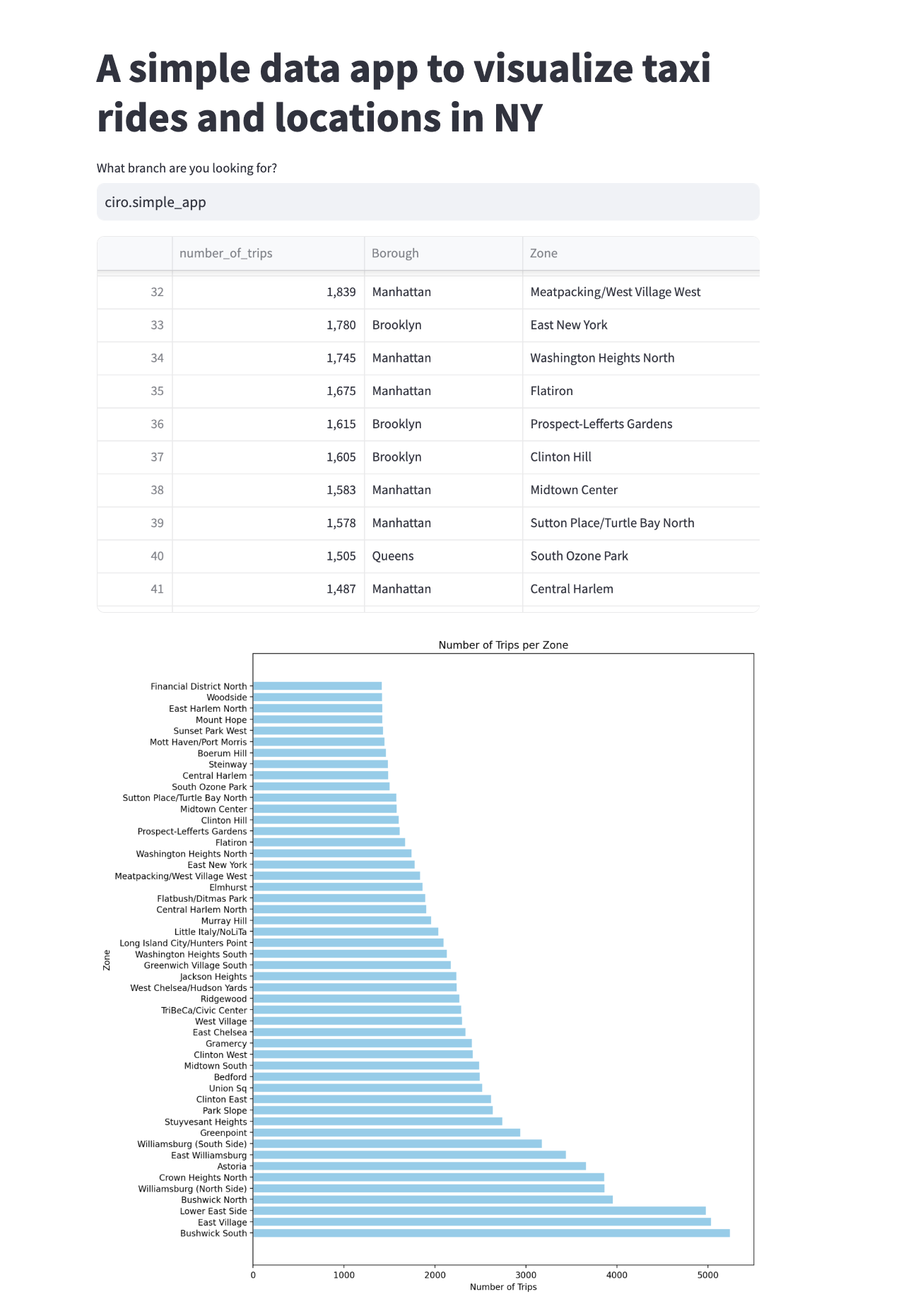
This app will simply visualize the final table of our pipeline, nothing fancy.

The programmable Lakehouse¶

One of the core strengths of bauplan is that every key operation on the platform can be seamlessly integrated into other applications using its straightforward Python SDK. Concepts such as plan creation, data import, execution, querying, branching, and merging—demonstrated throughout this documentation—are all accessible via simple SDK methods. This design makes your data stack highly programmable and easy to embed into any existing workflow, offering flexibility and efficiency for modern data-driven applications. This Streamlit app serves as a simple example of how Bauplan can be integrated into other applications using its Python SDK. In this example, we demonstrate the use of the query method, which allows bauplan to function as a query engine. With this method, we can run arbitrary SQL queries and seamlessly convert the results into a tabular objects (e.g. Pandas DataFrame). This enables us to perform real-time interactive queries on any table within any branch of the data catalog that we have access to, providing a powerful way to explore and visualize data in real time.

Summary¶

We have demonstrated how Bauplan can be used to develop a data pipeline that powers a simple data visualization app. Through straightforward abstractions, we achieved the following:

Created a branch in our data catalog.
Built a transformation pipeline leveraging multiple dependencies.
Materialized the pipeline’s results in the data lake as Iceberg tables.

Throughout the process, we did not need to manage runtime compute configurations, containerization, Python environments, or the persistence of data in the lake and catalog—Bauplan handled all of that seamlessly. Moreover, with a simple import statement, we integrated the bauplan runtime into our Streamlit app. Thanks to the Bauplan Python SDK, embedding the platform’s capabilities into other applications is both intuitive and efficient.