ML Model Training and Deployment Pipeline
In this example, we demonstrate how to organize and run a simple machine learning project using Bauplan. We’ll create and execute a pipeline that:
Ingests raw data from the TLC NY taxi dataset.
Transforms the data into a training dataset with the appropriate features.
Trains a Linear Regression model to predict the tip amount for taxi rides.
Writes the predictions to an Iceberg table for further analysis.
Additionally, we’ll leverage the Bauplan SDK within notebooks to explore both the dataset and the generated predictions interactively. This project highlights how Bauplan simplifies building end-to-end machine learning workflows.
Set up
In this example, we will use Jupyter Notebooks, so we will need to install the right dependencies. Go into the example folder, and create a virtual environment.
python -m venv venv
source venv/bin/activate
pip install -r requirements.txt
Make sure you have a bauplan_project.yml file with a unique project id, and a project name.
project:
    id: a8133e8c-5abd-490a-b12e-223abaf60981
    name: machine-learning-regression
Exploratory analysis
The first step is to explore the dataset using one of our notebooks to identify the best features for training the model. This process is straightforward with the help of our SDK.
Launch Jupyter Lab and open the notebook feature_exploration.ipynb. The code in the notebook is well-commented, so you can follow along and understand the feature selection process directly from the code.
cd 03-ml-regression-model
venv/bin/jupyter lab
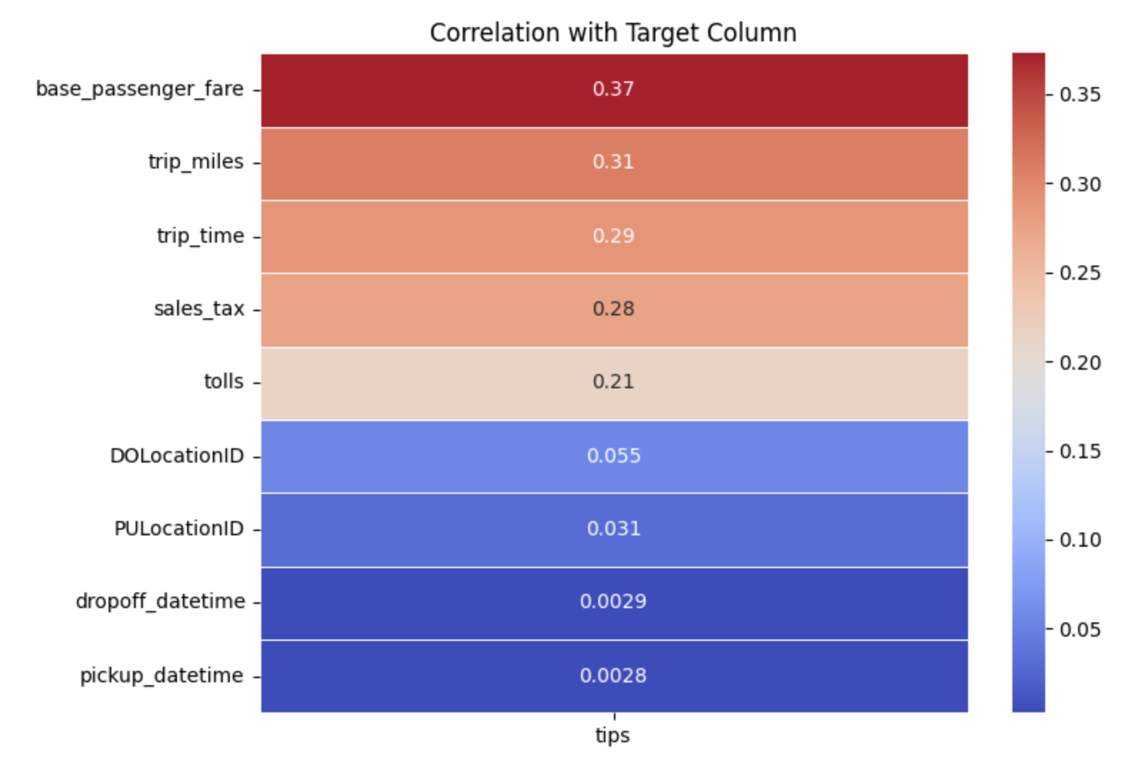
In the notebook, we extract a sample of data from the taxi_fhvhv table and compute a correlation matrix. We then display a heatmap to identify which features have the strongest correlation with our target variable, tips.
The top features identified are base_passenger_fare, trip_miles, and trip_time, which we will use as input columns to train the Linear Regression model.
The pipeline
This pipeline retrieves raw data from a data lake and processes it to train a Linear Regression model that predicts the tip amount for the length of taxi rides.
Run the pipeline
First, create a new branch and switch to it.
bauplan branch create <YOUR_BRANCH>
bauplan branch checkout <YOUR_BRANCH>
With the new branch checked out, make sure you are in the right folder and run the pipeline to materialize our predictions.
cd pipeline
bauplan run
Prepare the training dataset
Your pipeline consists of two main operations that work together to prepare taxi trip data for machine learning. The first operation uses the clean_taxi_trips function to handle data retrieval. This function connects to your data source through a Python S3 scan, accessing the taxi_fhvhv table to extract ten essential columns. It specifically filters the data based on pickup_datetime, pulling six months of historical data that amounts to roughly 19GB. As you work with this substantial dataset, you’ll get a clear sense of how bauplan manages data retrieval at scale.
Note
For more rapid development cycles, you can always use the bauplan run --dry-run command to test your workload in-memory.
The second operation focuses on transforming this raw data into a format suitable for machine learning models. Rather than working with all retrieved columns, this function processes only the specific columns declared in the input model definition. Using a combination of Pandas and Scikit-Learn, it creates a normalized dataset ready for model training.
Important
One particular transformation worth noting involves the trip_miles feature, which undergoes log-normalization to achieve a more balanced distribution. Additionally, all features are rescaled to ensure they contribute equally to the model’s learning process, preventing any unintended bias that might arise from differing measurement scales.
import bauplan

@bauplan.model()
# for this function we specify one dependency, Pandas 2.2.0
@bauplan.python('3.11', pip={'pandas': '2.2.0'})
def clean_taxi_trips(
        data=bauplan.Model(
            'taxi_fhvhv',
            # this function performs an S3 scan directly in Python, so we can specify the columns and the filter pushdown
            # by pushing the filters down to S3 we make the system considerably more performant
            columns=[
                'pickup_datetime',
                'dropoff_datetime',
                'PULocationID',
                'DOLocationID',
                'trip_miles',
                'trip_time',
                'base_passenger_fare',
                'tolls',
                'sales_tax',
                'tips'],
            filter="pickup_datetime >= '2023-01-01T00:00:00-05:00' AND pickup_datetime < '2023-03-31T00:00:00-05:00'"
        )
):
    import math
    import pandas as pd

    # debugging lines to check print the version of Python interpreter and the size of the table
    size_in_gb = data.nbytes / math.pow(1024, 3)
    print(f"This table is {size_in_gb} GB and has {data.num_rows} rows")

    # input data is always an Arrow table, so if you wish to use pandas, you need an explicit conversion
    df = data.to_pandas()

    # exclude rows based on multiple conditions
    df = df[(df['trip_miles'] > 1.0) & (df['tips'] > 0.0) & (df['base_passenger_fare'] > 1.0)]

    # output the data as a Pandas dataframe
    return df

@bauplan.model()
@bauplan.python('3.10', pip={'pandas': '1.5.3', 'scikit-learn': '1.3.2'})
def training_dataset(
        data=bauplan.Model(
            'clean_taxi_trips',
        )
):
    import pandas as pd
    import numpy as np
    from sklearn.preprocessing import StandardScaler

    # convert data from Arrow to Pandas
    df = data.to_pandas()

    # drop all the rows with NaN values
    df = df.dropna()
    # add a new column with log transformed trip_miles to deal with skewed distributions
    df['log_trip_miles'] = np.log10(df['trip_miles'])
    # define training and target features
    features = df[['log_trip_miles', 'base_passenger_fare', 'trip_time']]
    target = df['tips']
    pickup_dates = df['pickup_datetime']

    # scale the features to ensure that they have similar scales
    # compute the mean and standard deviation for each feature in the training set
    # then use the computed mean and standard deviation to scale the features.
    scaler = StandardScaler()
    scaled_features = scaler.fit_transform(features)
    scaled_df = pd.DataFrame(scaled_features, columns=features.columns)
    scaled_df['tips'] = target.values # Add the target column back to the DataFrame
    scaled_df['pickup_datetime'] = pickup_dates.values  # Add the date column back to the DataFrame

    # print the size of the training dataset
    print(f"The training dataset has {len(scaled_df)} rows")

    # The result is a new array where each feature will have a mean of 0 and a standard deviation of 1
    return scaled_df
Train the model
Training a model can be seamlessly integrated into the pipeline, just like any other step, by executing arbitrary code within a bauplan model. The train_linear_regression function uses Scikit-Learn to prepare the train, validation, and test sets, separating the training features from the target feature.
Once the dataset is split, we train the model using Scikit-Learn’s built-in LinearRegression method, ensuring a straightforward and efficient training process.
Passing ML models across functions
bauplan models are functions from and to tabular artifacts, like tables and dataframes. The general structure of a data pipeline in bauplan consists of a sequence of functions that take a table-like object as input and return a table-like object as output.
For users, this is the only key constraint: as long as each function adheres to this structure, everything else is handled by the system.
Developers can implement bauplan models using Python functions or SQL queries without worrying about how individual functions are executed or how data is passed across them.
As long as the output is a table-like object—such as an Arrow Table, Pandas DataFrame, or list of dictionaries—the pipeline will run smoothly.
In addition to handling tables, Machine Learning workflows often involve models, which must be passed between functions.
bauplan provides a built-in utility, bauplan.store (see the reference documentation), to persist and retrieve models from a key-value store.
This feature makes it easy to pass trained models between functions in a pipeline.
The entire code for training and testing a Linear Regression model is the following. It is heavily commented, so you can read through it to get a clear understanding of how it works.
This is not the only design pattern for Machine Learning. For instance, we could decide to serialize the model and save it as a file to retrieve it later on in the pipeline or even use a more sophisticated system like a feature store. Ultimately, the framework is powerful enough to allow for more complex designs. For now, it is enough to know that bauplan.store provides a simple way to pass a ML model across bauplan functions in a DAG.
@bauplan.model()
# for this function we specify two dependencies, Pandas 2.2.0 and Scikit-Learn 1.3.2
@bauplan.python('3.11', pip={'pandas': '2.2.0', 'scikit-learn': '1.3.2'})
def train_regression_model(
        data=bauplan.Model(
            'training_dataset',
        )
):
    from sklearn.model_selection import train_test_split
    from sklearn.linear_model import LinearRegression

    # convert arrow input into a Pandas DataFrame
    df = data.to_pandas()

    # Define the training and validation set sizes
    training_threshold = 0.8
    validation_threshold = 0.1  # This will implicitly define the test size as the remaining percentage
    # Split the dataset into training and remaining sets first
    train_set, remaining_set = train_test_split(df, train_size=training_threshold, random_state=42)
    # Split the remaining set into validation and test sets
    validation_threshold_adjusted = validation_threshold / (1 - training_threshold)
    validation_set, test_set = train_test_split(remaining_set, test_size=validation_threshold_adjusted, random_state=42)
    #print(f"The training dataset has {len(train_set)} rows")
    print(f"The validation set has {len(validation_set)} rows")
    print(f"The test set has {len(test_set)} rows (remaining)")

    # prepare the feature matrix (X) and target vector (y) for training
    X_train = train_set[['log_trip_miles', 'base_passenger_fare', 'trip_time']]
    y_train = train_set['tips']
    # Train the linear regression model
    reg = LinearRegression().fit(X_train, y_train)

    # persist the model in a key, value store so we can use it later in the DAG
    from bauplan.store import save_obj
    save_obj("regression", reg)

    # Prepare the feature matrix (X) and target vector (y) for validation
    X_test = validation_set[['log_trip_miles', 'base_passenger_fare', 'trip_time']]
    y_test = validation_set['tips']

    # Make predictions on the validation set
    y_hat = reg.predict(X_test)
    # Print the model's mean accuracy (R^2 score)
    print("Mean accuracy: {}".format(reg.score(X_test, y_test)))

    # Prepare the output table with predictions
    validation_df = validation_set[['log_trip_miles', 'base_passenger_fare', 'trip_time', 'tips']]
    validation_df['predictions'] = y_hat

    # Display the validation set with predictions
    print(validation_df.head())

    return test_set

@bauplan.model(materialization_strategy='REPLACE')
# for this function we specify two dependencies, Pandas 2.2.0 and Scikit-Learn 1.3.2
@bauplan.python('3.11', pip={'scikit-learn': '1.3.2', 'pandas': '2.1.0'})
def tip_predictions(
        data=bauplan.Model(
            'train_regression_model',
        )

):

    # retrieve the model trained in the previous step of the DAG from the key, value store
    from bauplan.store import load_obj
    reg = load_obj("regression")
    print(type(reg))

    # convert the test set from an Arrow table to a Pandas DataFrame
    test_set = data.to_pandas()

    # Prepare the feature matrix (X) and target vector (y) for test
    X_test = test_set[['log_trip_miles', 'base_passenger_fare', 'trip_time']]
    y_test = test_set['tips']

    # Make predictions on the test set
    y_hat = reg.predict(X_test)
    # Print the model's mean accuracy (R^2 score)
    print("Mean accuracy: {}".format(reg.score(X_test, y_test)))

    # Prepare the finale output table with the predictions
    prediction_df = test_set[['log_trip_miles', 'base_passenger_fare', 'trip_time', 'tips']]
    prediction_df['predictions'] = y_hat

    # return the prediction dataset
    return prediction_df
Explore the results
Once the predictions generated by the model are materialized in the data catalog as an Iceberg table, we can leverage the bauplan SDK to integrate the table into exploration tools, such as notebooks, or into a visualization app.
To assess the accuracy of our predictions, we use various types of plots in the notebook, employing Matplotlib and Seaborn for data visualization. As usual, we interact with the data directly from our branch of the data catalog using the bauplan SDK’s query method.
Launch Jupyter Lab again, and open the prediction_visualization.ipynb notebook to explore the prediction results.
cd 03-ml-regression-model
venv/bin/jupyter lab
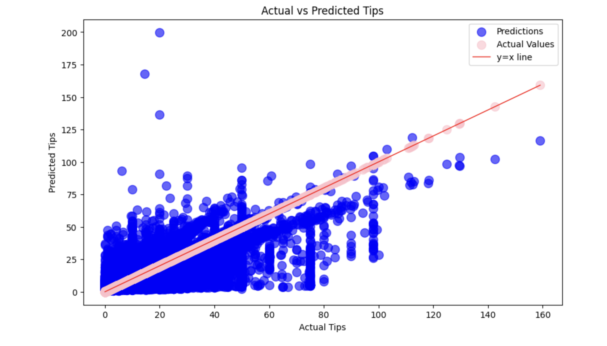
We will use three different plots to evaluate the performance of the Linear Regression model we just trained: Actual vs. Predicted Values Plot: this scatter plot compares the predicted values with the actual values. Ideally, the points should align closely along the line y = x, indicating accurate predictions.
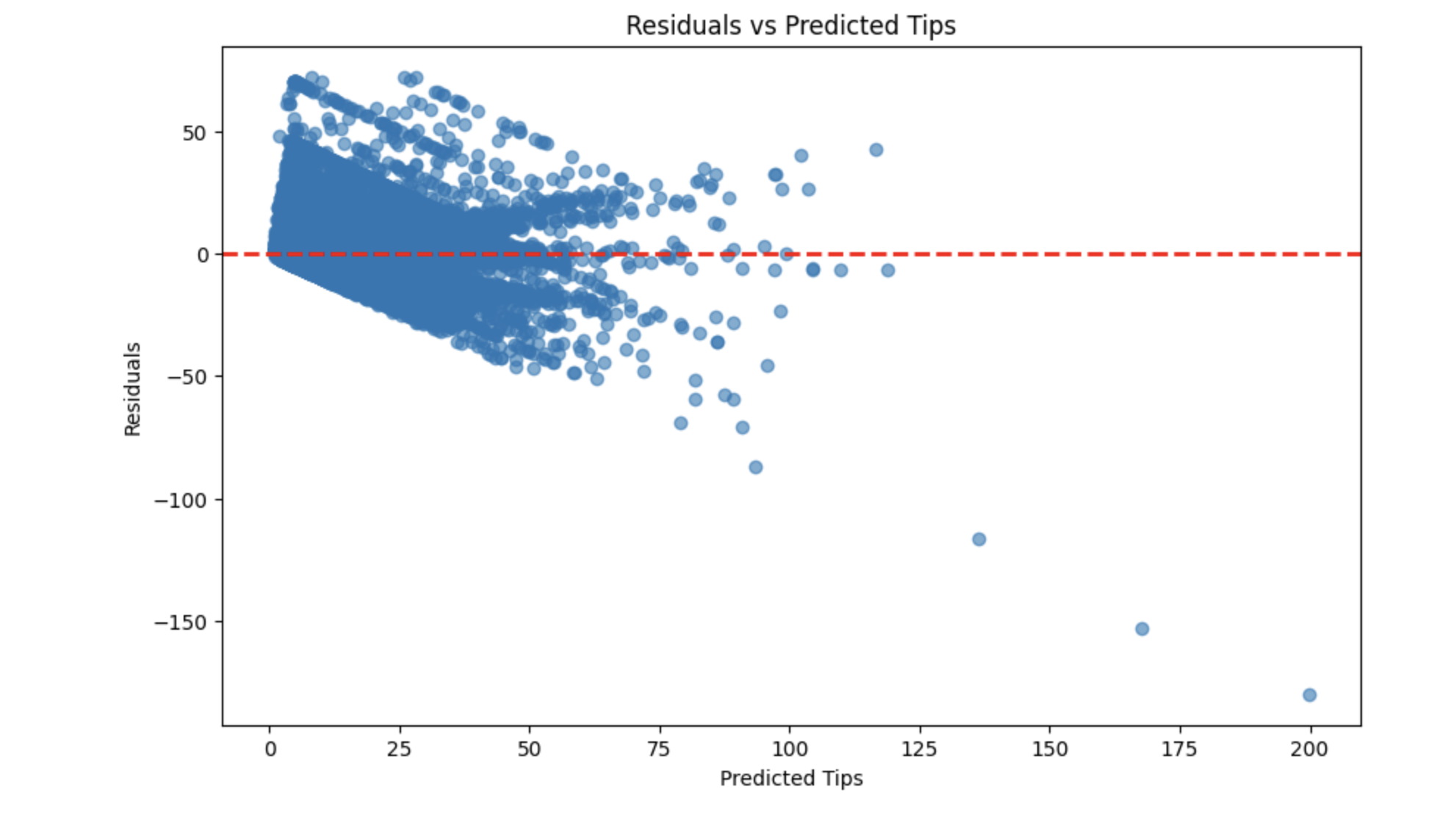
Residual Plot: This plot shows the residuals (differences between actual and predicted values) against the predicted values. Ideally, the residuals should be randomly distributed around zero, indicating that the model captures the underlying patterns in the data.
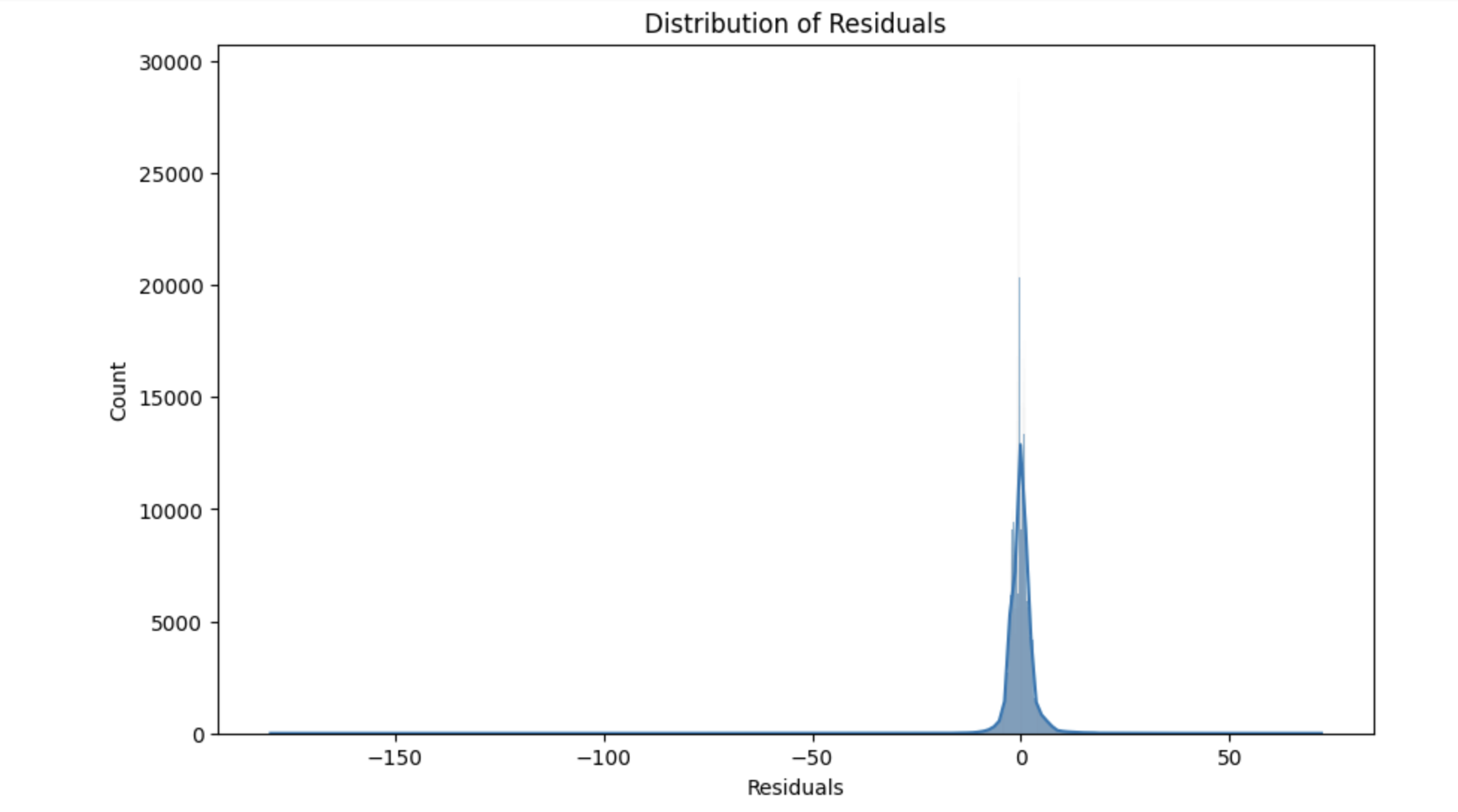
Distribution of Residuals: This histogram shows the distribution of the residuals. Ideally, the residuals should be normally distributed around zero.
The code in there is heavily commented, so you can explore it directly in the notebook.
Summary
In this chapter:
We demonstrated how to use Bauplan to build a machine learning pipeline that predicts the tip amount for taxi rides.
We explored the dataset, prepared the training data, trained a Linear Regression model, and visualized the predictions.
This example showcases bauplan’s flexibility and ease of use in integrating machine learning workflows seamlessly into data pipelines.